Tutorial: AENET Training Pipeline
In this tutorial, we use the N2 dimer as an example to explain the complete procedure for creating training data from first-principles calculations (Quantum ESPRESSO) and building a machine learning potential with AENET.
The sample files are located in sample/aenet_training/.
Workflow Overview
1. Structure Generation (relax/)
   └→ Generate random N2 dimer structures
   └→ Compute energies and forces with QE (SCF)

2. Training Data Creation (relax/)
   └→ Extract energies and forces from QE output
   └→ Generate training data in XSF format

3. Fingerprint Generation (generate/)
   └→ Compute atomic descriptors with AENET generate.x

4. Neural Network Training (train/)
   └→ Train the potential with AENET train.x

5. Prediction and Validation (predict/)
   └→ Predict energies of test structures with AENET predict.x
   └→ Compare with QE calculations
Step 1: Structure Generation
Work in the sample/aenet_training/relax/ directory.
structure_make.py randomly generates N-N bond distances in the range of 0.5 to 2.0 Angstrom
and creates Quantum ESPRESSO input files.
Note
A pseudopotential file (N.pbe-n-kjpaw_psl.1.0.0.UPF) is required in each directory.
When using run_all.sh, it is downloaded automatically.
For manual execution, place it in the relax/pseudo_Potential/ directory.
import random
structure_list = []
for i in range(20):
    structure_list.append(random.uniform(0.5, 2.0))
The template file (template.txt) is in QE input format, where value_01 is
the placeholder for the N-N bond distance:
&CONTROL
  calculation = 'scf'
  tprnfor     = .true.
  pseudo_dir  = './'
  outdir      = './'
/
&SYSTEM
  ntyp = 1, nat = 2, ibrav = 0
  ecutwfc = 44, ecutrho = 320
  occupations = 'smearing'
  smearing    = 'mp'
  degauss     = 0.01
/
...
ATOMIC_POSITIONS angstrom
  N 0.00 0.00 0.00
  N 0.00 0.00 value_01
Note
calculation='scf'performs a single-point calculation (no structural relaxation) at each geometry. This is used to obtain energies and forces at various randomly generated N-N distances.tprnfor=.true.enables printing of forces acting on atoms. Both energy and forces are required for AENET training data (XSF files), so this option must be specified.
Execution:
python3 structure_make.py
This generates directory_0/ through directory_19/, each containing a QE input file.
Run QE in each directory:
pw.x < n2_dimer.pwi > n2_dimer.pwo
Step 2: Training Data Creation
Extract energies and interatomic forces from the QE output files and convert them to AENET’s XSF format.
teach_data_make.py uses ASE’s ase.io.read() to read QE output files and
extracts energies (eV), atomic coordinates (Angstrom), and forces (eV/Angstrom),
outputting them in XSF format.
cd directory_0
python3 ../teach_data_make.py --input n2_dimer.pwo --output-dir teach_data
Output example (teach_data_1.xsf):
# total energy = -767.51 eV

ATOMS
N   0.00000000   0.00000000   0.00000000   0.00000000   0.00000000  -12.34567890
N   0.00000000   0.00000000   1.04970000   0.00000000   0.00000000   12.34567890
Step 3: Fingerprint Generation
Work in the sample/aenet_training/generate/ directory.
In generate.in, specify the paths to the training data and the atomic species:
OUTPUT N2.train

TYPES
1
N 389.83

SETUPS
N N.fingerprint.stp

FILES
20
../relax/directory_0/teach_data/teach_data_1.xsf
../relax/directory_1/teach_data/teach_data_1.xsf
...
Description of each keyword:
OUTPUT: Output file name. Binary file storing the fingerprint data (here,
N2.train)TYPES: Number of atomic species (next line) and, for each species, the element symbol and atomic energy shift value in eV (
N 389.83)SETUPS: Fingerprint setup file for each atomic species (
N.fingerprint.stp)FILES: Number of training data XSF files (next line) and the path to each file
N.fingerprint.stp is a fingerprint (structural descriptor) configuration file
that defines how the local atomic environment is transformed into input for the neural network.
It is required as input to generate.x.
For details on the file format, see the
AENET official documentation.
Example configuration for an N2 dimer:
DESCR
  Structural fingerprint setup for N-N in linear nitrogen molecule
END DESCR

ATOM N

ENV  1
N

RMIN 0.5

SYMMFUNC type=Behler2011
9
G=2 type2=N   eta=0.001  Rs=0.0  Rc=3.0
G=2 type2=N   eta=0.01   Rs=0.0  Rc=3.0
G=2 type2=N   eta=0.1    Rs=0.0  Rc=3.0
G=4 type2=N  type3=N   eta=0.001 lambda=-1.0  zeta=4.0 Rc=3.0
G=4 type2=N  type3=N   eta=0.001 lambda=1.0   zeta=4.0 Rc=3.0
G=4 type2=N  type3=N   eta=0.01  lambda=-1.0  zeta=4.0 Rc=3.0
G=4 type2=N  type3=N   eta=0.01  lambda=1.0   zeta=4.0 Rc=3.0
G=4 type2=N  type3=N   eta=0.1   lambda=-1.0  zeta=4.0 Rc=3.0
G=4 type2=N  type3=N   eta=0.1   lambda=1.0   zeta=4.0 Rc=3.0
Description of each keyword:
ATOM: The central atom element for which fingerprints are computed (here, N)
ENV: Number of species in the environment and their symbols. N2 is a single-species system, so 1 (N only)
RMIN: Minimum interatomic distance (Angstrom). Structures with shorter distances are excluded
SYMMFUNC type=Behler2011: Uses Behler’s symmetry functions [J. Behler, J. Chem. Phys. 134, 074106 (2011)]
G=2 (radial functions): Descriptors depending on two-body distances
eta: Width of the function. Smaller values give sharper functions, larger values give smoother onesRs: Shift of the function centerRc: Cutoff distance (Angstrom). Only atoms within this range are considered
G=4 (angular functions): Descriptors depending on three-body angles
eta: Radial widthlambda: +1 or -1. Controls the sign of the angular dependencezeta: Angular resolution. Larger values increase sensitivity to specific anglesRc: Cutoff distance (Angstrom)
Execution:
generate.x generate.in > generate.out
Output:
N2.train: Binary dataset for training
Step 4: Neural Network Training
Work in the sample/aenet_training/train/ directory.
Set the training parameters in train.in:
TRAININGSET N2.train
TESTPERCENT 10
ITERATIONS  3000

TIMING

bfgs

NETWORKS
# atom   network           hidden
# types  file-name         layers   nodes:activation
N        N.5t-5t.ann       2        10:tanh 10:tanh
Description of each keyword:
TRAININGSET: Fingerprint data file generated by
generate.x(here,N2.train)TESTPERCENT: Percentage of training data used for testing (here, 10%)
ITERATIONS: Number of weight optimization iterations (here, 3000)
TIMING: Print execution time for each iteration
bfgs: Weight optimization method. Choose from:
steepest_descent: Online steepest descentbfgs: BFGS quasi-Newton method (recommended)levenberg_marquardt: Levenberg-Marquardt method
NETWORKS: Neural network configuration. Each line specifies:
Element symbol of the atomic species (
N)Output ANN potential file name (
N.5t-5t.ann)Number of hidden layers (
2)Nodes and activation function for each hidden layer (
10:tanh 10:tanh)
Execution:
train.x train.in > train.out
Example of training results (from train.out):
Number of training structures :         18
Number of testing structures  :          2
Total number of weights       :        221
Atomic energy shift           :   -747.530391 eV
Output:
N.5t-5t.ann: Trained ANN potential file
Step 5: Prediction and Validation
Work in the sample/aenet_training/predict/ directory.
First, generate the test XSF files using generate_test_xsf.py.
This creates 201 structures with N-N distances from 0.00 to 2.00 Angstrom in 0.01 Angstrom increments:
python3 generate_test_xsf.py
This generates test XSF files in the predict_data_set_test/ directory.
Then, configure the prediction settings in predict.in:
TYPES
1
N

NETWORKS
  N  N.5t-5t.ann

FORCES

FILES
201
../predict_data_set_test/test_0.00.xsf
../predict_data_set_test/test_0.01.xsf
...
Description of each keyword:
TYPES: Number of atomic species (next line) and the element symbol for each species
NETWORKS: Trained ANN potential file for each atomic species (
N.5t-5t.ann)FORCES: Also predict forces (optional)
FILES: Number of XSF files to predict (next line) and the path to each file
Predict energies using the trained potential:
predict.x predict.in > predict.out
Visualization of Results
Use plot_distance_energy.py to create a plot comparing the predicted energies from the ANN potential
with the first-principles calculation results from QE:
python3 plot_distance_energy.py \
    --predict-out predict.out \
    --train-out ../train/train.out \
    --qe-dir ../relax \
    --n-structures 20 \
    --output distance_energy_plot.png
This script plots the following three datasets:
ANN prediction (blue): Interatomic distance vs. energy from
predict.outQE training data (red): Results from the SCF calculation XSF files
QE test data (green): Data points included in the test set from
train.out
In addition to the full-range plot (distance_energy_plot.png), a zoomed-in plot
around the potential minimum (distance_energy_plot_zoom.png, y-axis: -770 to -760 eV)
is also generated automatically.
Calculation Results
The following graph compares the predicted energies from the ANN potential with the first-principles calculation results from QE (zoomed in around the potential minimum).
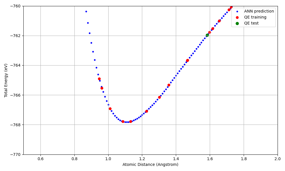
Energy-distance curve for the N2 dimer (zoomed in). Blue: ANN prediction, Red: QE training data, Green: QE test data.
Key results:
A Morse-type potential curve is reproduced, with the energy minimum (approximately -768 eV) near the equilibrium N-N distance (approximately 1.1 Angstrom)
The ANN potential reproduces the QE results well within the range of the training data (20 points)